“`html
Effective Ways to Find IQR for Analyzing Data in 2025
Understanding the Interquartile Range (IQR)
The **interquartile range (IQR)** is a pivotal statistical measure that describes the spread of a dataset. It is calculated by finding the difference between the upper and lower quartiles (Q3 and Q1). This range encapsulates the middle 50% of the data, providing significant insights into variability and **data dispersion** within a dataset. The importance of the IQR lies in its ability to represent the **IQR in descriptive statistics**, especially when compared to other measures of variability, such as the standard deviation or range. Understanding how to find **IQR** enhances your overall statistical knowledge, allowing you to interpret and analyze data efficiently.
What Does the IQR Represent?
The **IQR** offers a robust measure of variability by condensing the central portion of a dataset. This enables the researcher or analyst to focus on the data segment that holds the most meaning, minimizing the influence of outliers. When you are **calculating IQR**, you’re essentially determining the spread at which the middle half of your data resides. This information can be particularly valuable when visualizing data with a boxplot, where the IQR is illustrated as the box itself. Understanding the **statistical interpretation of IQR** can guide better data-driven decisions, enabling clear insights into the dataset’s distribution.
The Significance of the IQR in Data Analysis
The **IQR** plays a critical role in detecting **outliers**. By utilizing the IQR in conjunction with a boxplot, analysts can easily identify values that deviate significantly from the standard range of data behavior. This is achieved by marking any data points lying beyond 1.5 times the IQR above Q3 or below Q1 as outliers. This analytical perspective is fundamental within fields such as data science and research. Analyzing IQR helps in creating a more comprehensive understanding of dataset behavior while avoiding the misconceptions that can arise from solely relying on the mean or standard deviation. To effectively implement this, one must be adept at **finding IQR** values through practical application and statistical methods.
Calculating the IQR Step-by-Step
Calculating the IQR involves a systematic approach for obtaining Q1 and Q3 from a data set. This foundational knowledge is pivotal for anyone looking to delve deeper into **statistical methods IQR**. Each step of the calculation can enhance both your understanding of data and your analytical skills. Here’s how to meticulously carry out the IQR calculation:
Step 1: Organize Data
Begin by sorting your data in ascending order. This crucial first step ensures clarity in identifying the quartiles. For example, consider the dataset: {7, 15, 36, 39, 40, 41, 49, 56}. Once organized, we can effectively proceed to locate the quartiles.
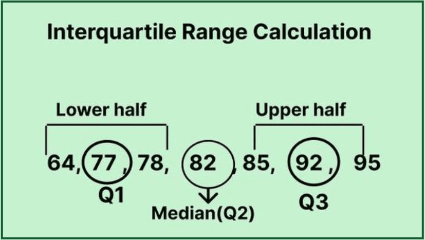
Step 2: Determine Quartiles
To find the quartiles, you need to split your sorted data into two halves: the lower half (excluding the median for odd datasets) and the upper half. For our example, the **lower quartile (Q1)** is the median of the first half, while the **upper quartile (Q3)** serves as the median of the second half. This process leads us to discover that Q1 = 36 and Q3 = 40, essential values in the **IQR formula**.
Step 3: Apply the IQR Formula
The final step is the calculation using the IQR formula: IQR = Q3 – Q1. In our example, the IQR would therefore be calculated as 40 – 36 = **4**. This result reveals the spread within the middle 50% of our data value ranges, offering insight into the data’s concentration.
Applications and Relevance of IQR
The IQR is not only a measure of variability but also holds multiple applications in interpreting data effectively. The **importance of IQR** stretches across various fields such as finance, academics, and market research. Utilizing IQR allows for a more focused approach when working with data and assists in facilitating clearer understanding and communication surrounding complex datasets.
IQR Usage in Different Contexts
In business analytics, the **IQR** can be instrumental in performance evaluation by filtering out anomalies that skew typical metrics. Similarly, research papers often utilize IQR to succinctly showcase the variability of datasets while emphasizing **IQR value comparisons**. This flexibility makes IQR a preferred method in both qualitative and quantitative analysis settings.
IQR Visualization and Its Importance
Visual representation of IQR is often done through boxplots, a powerful tool for depicting data distributions at a glance. A **box and whisker plot analysis** effectively communicates the IQR alongside the median and possible outliers. This visual method promotes deeper insights into the dataset’s structure, creating a more intuitive understanding of underlying data behavior. Analyzing how to depict the data through these methods enhances the **statistical significance of IQR** in portraying not just central tendencies, but the variability as well.
Key Takeaways
- The **IQR** represents data spread and is crucial for finding outliers and understanding variability.
- Calculating the IQR involves organizing your data, identifying quartiles, and applying the IQR formula.
- IQR is widely used across many fields for reliable data analysis and representation.
- Utilizing IQR visualizations like boxplots offers profound insights into data distributions.
- The IQR lays foundational knowledge in statistics, improving decision-making through analytical proficiency.
FAQ
1. What is the IQR definition, and why is it important?
The **IQR**, or interquartile range, is defined as the difference between the first quartile (Q1) and the third quartile (Q3) in a dataset. Its importance lies in its ability to measure statistical dispersion while minimizing outlier impact. This makes it particularly valuable in fields requiring precise data interpretation, as it effectively summarizes the range within which the central 50% of the data resides, highlighting its relevance as a statistical tool.
2. How does IQR help in detecting outliers?
The **IQR** assists in outlier detection by marking data points that lie outside the established boundaries of Q1 – 1.5*IQR and Q3 + 1.5*IQR. Any values below this lower limit or above this upper limit are considered potential outliers. This systematic approach allows for cleaner and more accurate data analysis, essential for maintaining data integrity and resulting insights that drive informed decisions.
3. Can IQR be used with different types of datasets?
Yes, the **IQR** can be applied across various datasets, ranging from numerical values in scientific research to financial data in business settings. Its versatility makes it an excellent tool for analyzing disparate data, providing consistent insights on variance regardless of the data’s context. Whether you’re working with **IQR in quantitative analysis** or more complex models, its calculation remains a fundamental aspect of thorough data examination.
4. What are the advantages of using IQR compared to standard deviation?
One major advantage of employing the **IQR** over standard deviation is its resistance to the influence of outliers. The IQR focuses solely on the middle 50% of the dataset, while standard deviation considers every data point. This characteristic makes the IQR particularly suitable for datasets with significant outliers or non-normal distributions, helping to provide a clearer perspective on the data’s **distribution shapes**.
5. How can I visualize IQR data effectively?
Effective visualization of IQR data is often achieved using boxplots, where the central box represents the IQR while markers highlight outliers. Additionally, using scatter plots or strip charts can help to depict the spread, patterns, and **dispersion characteristics** of the dataset visually. By leveraging these graphical representations, analysts can communicate their findings and insights more clearly to stakeholders and audiences.
6. Can you provide a practical IQR example?
Sure! Consider a dataset of exam scores: {55, 60, 65, 70, 75, 80, 85, 90, 95, 100}. Upon sorting, we find Q1 (where the lower 25% of scores lie) as 67.5 and Q3 as 92.5. Thus, **IQR = Q3 – Q1 = 25%.** This IQR indicates that the middle 50% of scores range between 67.5 and 92.5, offering insights into overall performance distribution and identifying how tight or dispersed the scores may be.
“`